Neural Discrete Representation Learning

Abstract

• discrete representation
  • to prevent “posterior collapse”
• learnt prior distribution

Motivation

• Goal: optimize $p_θ(x)$ while conserves the important features of the data in the latent space
• existing VAE models suffer from “posterior collapse”
  • what is the “posterior collapse” ?
    • please refer Discussion #1. ¹

 

VQ-VAE

Discrete Latent Variables

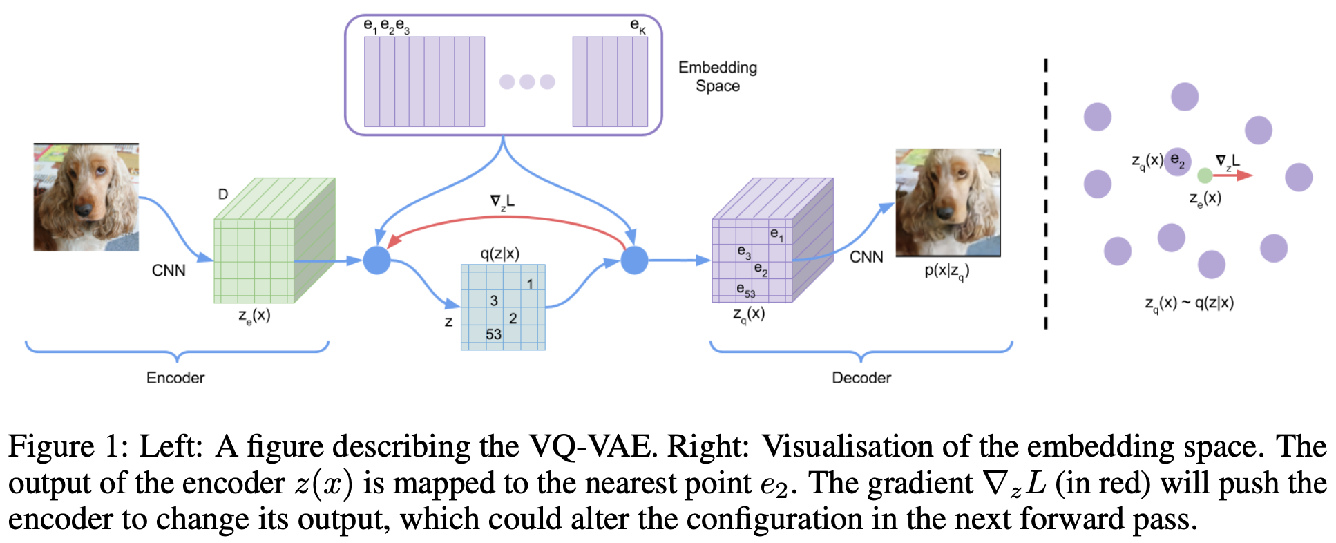
• each input is encoded into $z_e(x)$

• then each embedding vector is calculated into $e\in ℝ^{K\times D}$ by nearest neighbor lookup

• $q(z|x)$ are defined as:

$$ q(z = k \mid x) = \begin{cases} 1 & \text{for } k = \arg\min_j \| z_e(x) - e_j \|_2, \\ 0 & \text{otherwise} \end{cases} $$

• $q(z=k|x)$ is deterministic

  • let $p(z)$ a uniform over $z$
  • $D_{KL}$ is constant and equal to $\log K$

• In conclusion, the discretization process is as follows:

$$ z_q(x) = e_k, \quad \text{where} \quad k = \arg\min_j \| z_e(x) - e_j \|_2 $$

Learning

• Gradient cannot be defined on discretization process
• Approximate grad by straight-through estimator and copying grad
• To calculate grad, calculated grad from the decoder $\nabla_z L$ is passes to the encoder

$$ L = \log p(x \mid z_q(x)) + \|\text{sg}[z_e(x)] - e\|_2^2 + \beta \|z_e(x) - \text{sg}[e]\|_2^2 $$

About the Loss

• Reconstruction Loss (first term)
  • reconstruct $x$ from quantized $z_q(x)$
• Codebook Loss (second term)
  • let the codebook entry $e$ to be close to the $z_e(x)$
  • what is the stop grad?
    • we cannot compute the loss directly from $q_φ(z_q(x)|x)$
    • $x$ and $z_q(x)$ has no grad connection
    • We gotta train by codebook loss
    • However, if we design the loss like $\|z_e-e\|^2_2$, it will not converge since two moves together
      • why?
        • if two moves simultaneously, they may miss each other
        • it’s like chasing each other’s tails

General

• the first term of the loss equation is reconstruction term $\log p(x|z_q(x))$

  • It is not connected to $z_e(x)$
  • the dictionary learning algorithm is the Vector Quantization (VQ) algorithm

• VQ calculates L2 error between $e_i$ to $z_e(x)$ (second term)

  • $e_i$ stands for the embdding
  • $sg$ stands for the stopgradient operator that is defined as identity at forward computation time and has zero partial derivatives
  • TL;DR: since it is not possible to calculate the distance between $z_e(x)$ and $e$, the term is divided into two term and calculated individually.
• $$\log p(x) = \log \sum_k p(x|z_k)p(z_k)$$

• The decoder can be trained after VQ mapping is fully converged. (Discussion #3)

Prior

• prior distribution $p(z)$ is a categorical distribution
• While training VQ-VAE, the prior is kept constant and uniform
• After training, z is fit to an autoregressive distributuion $p(z)$ so that that can generate $z$ by ancestral sampling.
• But how does this prior prevent the posterior collapse problem? Discussion #2 ²
• What kind of generative modeling is VQ-VAE? Discussion #3 ³

 

Experiments

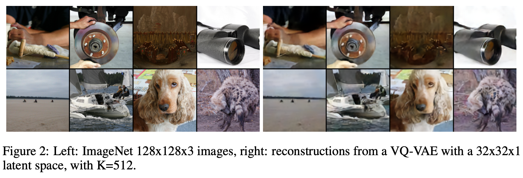
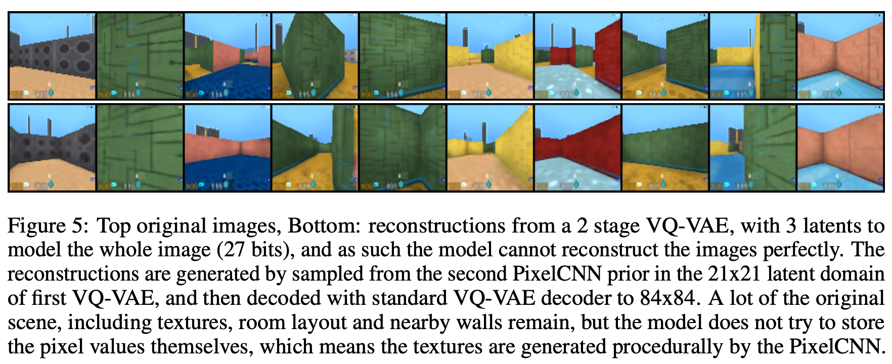
Images

• Image $x\in ℝ^{128×128×3}$
• Latent $z\in ℝ^{32×32×1}$ (with K=512)
• Reduction of $\frac{128×128×3×8}{32×32×9} \approx 42.6$ in bits. (Question #5)
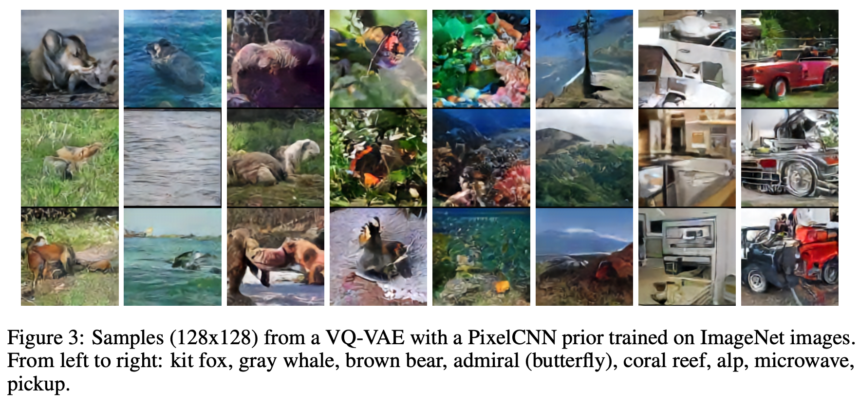
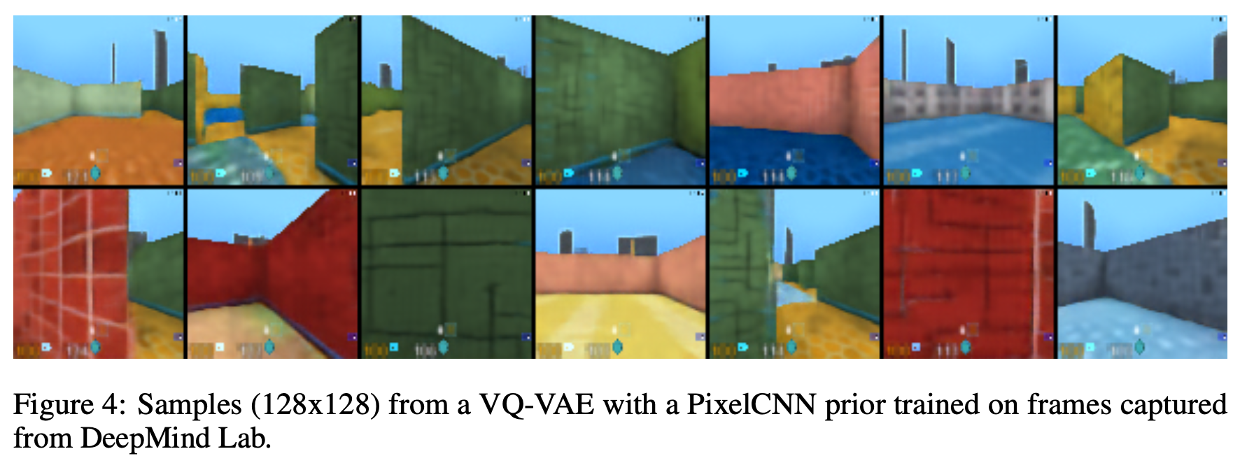
• Used PixelCNN prior

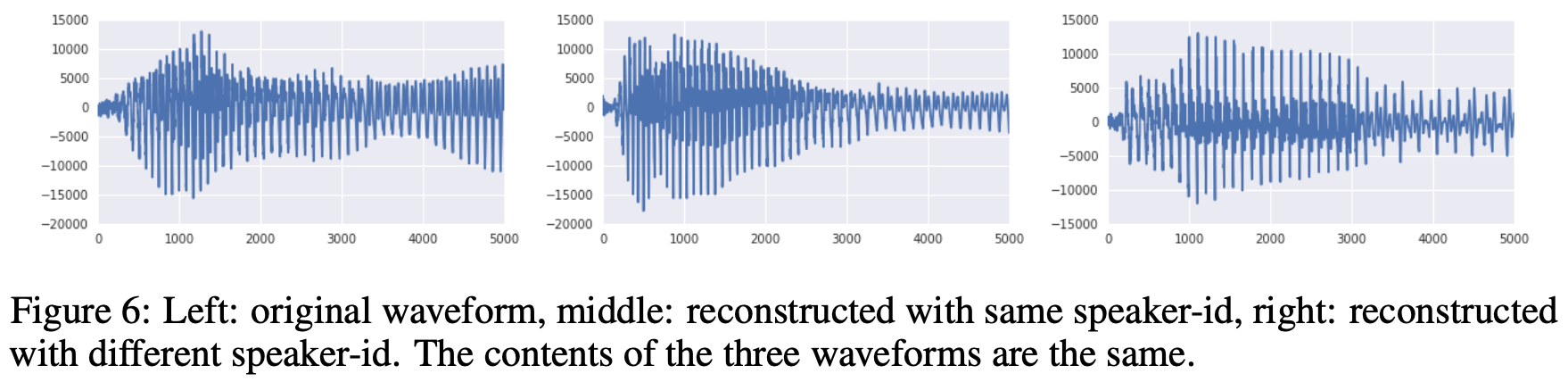
Audio

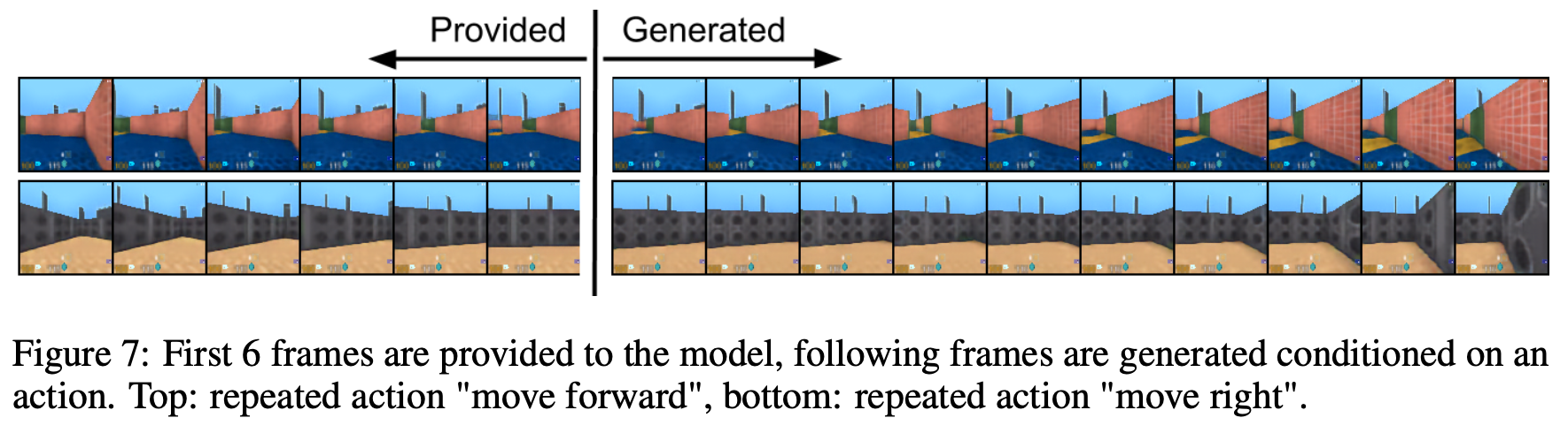
Video

Discussion

• In the VAE, if the decoder is super strong, than it may be able to generate a random average-looking image to minimize the loss
• Then the encoder fail to learn $q_φ(z|x)$, it just learn $p(z)$

• the encoder of the VQ-VAE is not a probabilistic model.
  • So there’s no such $q_φ(z|x)$
  • Since the output is not a pdf, there’s no KL divergence neither

• VQ-VAE is explicit, intractable generative model

  • It explicitly design the $p_θ(x)$
    • $$\log p(x) \approx \log p(x|z_q(x))p(z_q(x))$$
    • From Jensen’s inequality, $\log p(x)\ge \log p(x|z_q(x))p(z_q(x))$
  • The encoder and the decoder are determisitic functions
    • can be interpreted as the dirac delta function
  • the stochasity is implemented in sampling $z$
    • It is autoregressively sampling in ancestral sampling by PixelCNN
    • $p(z)$, which is modeled by PixelCNN, is very complicated and not tractable

• why log k?

• Question #5 What is the meaning of 8 and 9 in the formula?